Introductory Example

Introductory Example

This example illustrates the basic functionality of the toolbox and shows how the generated code and the interfaces are used. More details can be found in the user guide.

Problem Specification

Let us consider the following parametric problem (the parametric problem data is indicated in red).

$%note: \param is specified in configuration settings (plugin>>latex>>preamble), because not allowed to use new-c-ommand here (even not in comment) \begin{align*} \textrm{min}\quad &\tfrac{1}{2} x^T \underbrace{\text{diag}([1,2,3,4])}_{H} x + \param{g}^T x \\ \textrm{s.t.}\quad &x \in \mathcal{X}=\mathcal{X}_1\times\mathcal{X}_2 \\ &\underbrace{[0,1,-1,0]}_{A_{e}}\,x = \param{b_{e}} \end{align*}$

where $\mathcal{X}_1$ is a rotated box given by

$\begin{align*} &\mathcal{X}_1 =\Biggl\{x\in\mathbb{R}^2\left|\right. x=\underbrace{\begin{bmatrix}\cos\left(\frac{\pi}{6}\right)&-\sin\left(\frac{\pi}{6}\right)\\\sin\left(\frac{\pi}{6}\right)&\cos\left(\frac{\pi}{6}\right)\end{bmatrix}}_{R} v, \underbrace{\begin{bmatrix}-1\\0.5\end{bmatrix}}_{l}\leq v \leq \underbrace{\begin{bmatrix}1\\2\end{bmatrix}}_{u}, v\in\mathbb{R}^2\Biggr\} \end{align*}$

and $\mathcal{X}_2$ is a shifted Euclidean ball given by

$\begin{align*} &\mathcal{X}_2 =\Biggl\{x\in\mathbb{R}^2\left|\right.x=v+\underbrace{\begin{bmatrix}1\\-1\end{bmatrix}}_{s}, \|v\|\leq \param{r}, v\in\mathbb{R}^2 \Biggr\} \end{align*}$

Using FiOrdOs syntax, this problem is specified as follows. Note that the value 'param' defines a problem data to be parametric.

X1 = EssBox(2, 'l',[-1;0.5], 'u',[1;2], 'rot',[cos(pi/6),-sin(pi/6);sin(pi/6),cos(pi/6)]);
X2 = EssBall(2, 'r','param', 'shift',[1;-1]);
X  = SimpleSet(X1,X2);
op = OptProb('H',diag([1,2,3,4]), 'g','param', 'X',X, 'Ae',[0,1,-1,0], 'be','param');

Solver Setup and Code Generation

After specifying the problem, the solver is configured and finally C-code is generated. During the setup, default solver settings can be modified.

The procedure is as follows:

%instantiate solver
s = Solver(op,'approach','dual', 'algoOuter','gm', 'algoInner','fgm'); 
 
%optionally change settings, e.g.
%-maximum number of iterations
s.setSettings('algoOuter', 'maxit',100);
s.setSettings('algoInner', 'maxit',90);
%-gradient-map stopping criterion
s.setSettings('algoOuter', 'stopg',true, 'stopgEps',1e-3); 
s.setSettings('algoInner', 'stopg',true, 'stopgEps',1e-5);
 
%generate solver code  
s.generateCode('prefix','demo_');

Remarks:

Since the problem has an equality constraint, it is solved with the dual approach ('dual'), which uses two algorithms. In this example, the gradient method ('gm') is chosen as the outer algorithm to maximize the dual function ('algoOuter') whereas the fast gradient method ('fgm') solves the inner problem to determine the dual function's gradient ('algoInner').
'maxit' is the maximum number of iterations after which an algorithm terminates in any case.
By activating the gradient-map stopping criterion ('stopg'), an algorithm terminates if the norm of the gradient-map is below the specified accuracy ('stopgEps').
'prefix' defines the common prefix for the generated file names, interface functions and data types.
If you are not sure, which approach/algorithm(s) to choose, either let FiOrdOs decide (simply invoke s = Solver(op)) or let FiOrdOs display all possible approaches/algorithm(s) for your problem (command Solver.analyze(op)). For this problem, there is also the primal-dual approach available; it can be selected by s = Solver(op, 'approach', 'primal-dual')

The following table gives an overview on all generated files. The files in parentheses are created when executing the corresponding makefiles.

	filename	description
C-solver	`demo_solver.h`	solver interface
C-solver	`demo_solver.c`	solver implementation
Matlab interface	`demo_mex.c`	MEX source (wrapper for C-solver)
	`demo_mex_make.m`	makefile creating:
	(`demo_mex.mex*`)	-MEX-file
	`demo_mex.m`	Help file
Simulink interface	`demo_sfun.c`	S-Function source (wrapper for C-solver)
	`demo_sfun_make.m`	makefile creating:
	(`demo_sfun.mex*`)	-S-Function MEX-file
	(`demo_sfun_lib.mdl`)	-Simulink library (containing a masked subsystem block that encapsulates demo_sfun.mex*)
	`demo_sfun_lib_aux.m`	auxiliary file for demo_sfun_lib.mdl

Using the Solver in C

The interface defined in demo_solver.h consists of the two functions demo_init and demo_solve, which work on four structs of types demo_Params, demo_Settings, demo_Result, demo_Work.

The following C-program gives an example for how to use the interface. The program solves our problem for one specific realization of the parametric problem data.

demo_main.c

#include "demo_solver.h"
#include <stdio.h>
 
int main() {
 
  /* define and initialize the four structs */	
  demo_Params   params   = {0};
  demo_Settings settings = {0};
  demo_Result   result   = {0};
  demo_Work     work     = {0};
 
  demo_init(&params, &settings, &result, &work);	
 
 
  /* define all parametric data */
  params.g[0]    = 4;
  params.g[1]    = 3;
  params.g[2]    = 1;
  params.g[3]    = 2;
  params.be[0]   = 0.8;
  params.X2.r[0] = 1;
 
  /* optionally change some settings, e.g. */
  settings.algoOuter.maxit = 30;
 
  /* solve the problem */
  demo_solve(&params, &settings, &result, &work);
 
  /* use solution availabe in struct result */
  printf("d:    %g\n", result.d);
  printf("iter: %d\n", result.iter);
 
  return 0;
}

Note that the struct settings contains all solver settings that can be modified at runtime. They are initialized by demo_init to the values defined during the solver setup in Matlab.

The following code gives an example for compiling and linking the main file demo_main.c and the solver demo_solver.c in Linux. Finally, the resulting executable called demo is run.

gcc demo_main.c demo_solver.c -lm -o demo
./demo

Using the Solver in Matlab

Invoking the makefile by

demo_mex_make()

builds the binary MEX-file demo_mex.mex*, which then can be called like any Matlab function.

The following Matlab code gives an example for how to use the MEX-file. The code solves our problem for one specific realization of the parametric problem data.

%define all parametric data
mparams      = struct();
mparams.g    = [4;3;1;2];
mparams.be   = 0.8;
mparams.X2.r = 1;
 
%optionally change some settings, e.g.
msetgs       = struct();
msetgs.algoOuter.maxit = 30;
 
%call MEX-file
mres = demo_mex(mparams,msetgs);
 
%use result
mres
mres.x

Remarks:

The Matlab structs mparams, msetgs, mres correspond to the C-structs params, settings, result.
Customized help for the Matlab interface, including templates for the structs mparams and msetgs, is availabe by typing
```
help demo_mex
```

Using the Solver in Simulink

Invoking the makefile by

demo_sfun_make()

builds the S-Function MEX-file demo_sfun.mex* and the Simulink library demo_sfun_lib.mdl.

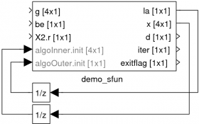
The library contains the following masked subsystem block, which can be instantiated by copying it into a Simulink model.

block	description
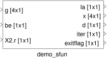	block inputs	parametric problem data
	mask parameters	solver settings sample time
	block outputs	results of optimization

Note that for some solver settings that can be accessed via the block mask, the data source can be configured as external. This means that the solver setting becomes a block input. As an example, this allows one to perform warm-starting as shown in the following figure.